Modeling Ironsworn’s core mechanic

Shawn Tomlin’s Ironsworn melds a number of different influences in a fresh way. Its core mechanic involves rolling an action die (a d6), adding a modifier, and comparing the result to two challenge dice (d10s). If the modified value from the action die is strictly greater than both challenge dice, the result is a strong success. If it is strictly greater than only one challenge die, the result is a weak success. If it is equal to or less than both challenge dice, it’s a failure.

A verbose way to model this is to enumerate the product of the three dice and then perform logical comparisons. expand can calculate the challenge-dice results for each action-die outcome. We can also deploy our prior counting trick for dealing with the two d10s.

>>> from dyce import H, HResult, expand
>>> from enum import IntEnum
>>> from typing import cast
>>> d6 = H(6)
>>> d10 = H(10)
>>> class IronResult(IntEnum):
...     FAILURE = 0
...     WEAK_SUCCESS = 1
...     STRONG_SUCCESS = 2
...
...     def __repr__(self) -> str:
...         return self.name  # makes formatting easier on the eyes
>>> def iron_dependent_term(action: HResult[int]) -> H[IronResult]:
...     res = 2 @ d10.lt(action.outcome)  # (1)!
...     return res.apply(IronResult)
>>> expand(iron_dependent_term, d6 + 1)  # expected results for an action modifier of +1
H({FAILURE: 271, WEAK_SUCCESS: 238, STRONG_SUCCESS: 91})

Our counting trick.

>>> action_mods = list(range(-1, 4))
>>> for action_mod in action_mods:
...     iron_distribution = expand(iron_dependent_term, d6 + action_mod)
...     print(f"{action_mod:+} -> {iron_distribution.format_short(include_avg=False)}")
-1 -> {FAILURE: 71.67%, WEAK_SUCCESS: 23.33%, STRONG_SUCCESS:  5.00%}
+0 -> {FAILURE: 59.17%, WEAK_SUCCESS: 31.67%, STRONG_SUCCESS:  9.17%}
+1 -> {FAILURE: 45.17%, WEAK_SUCCESS: 39.67%, STRONG_SUCCESS: 15.17%}
+2 -> {FAILURE: 33.17%, WEAK_SUCCESS: 43.67%, STRONG_SUCCESS: 23.17%}
+3 -> {FAILURE: 23.17%, WEAK_SUCCESS: 43.67%, STRONG_SUCCESS: 33.17%}

What’s with that 2 @ d10.lt(action.outcome)?

Let’s break it down. H(10).lt(value) will tell us how often a single d10 is less than value.

    >>> H(10).lt(5)  # how often a d10 is strictly less than 5
    H({False: 6, True: 4})

By taking advantage of the fact that, in Python, bools act like ints when it comes to arithmetic operators, we can count how often that happens with more than one interchangeable d10 by “summing” them.

    >>> d10_lt5 = H(10).lt(5)
    >>> d10_lt5 + d10_lt5
    H({0: 36, 1: 48, 2: 16})
    >>> (d10_lt5 + d10_lt5).total
    100

How do we interpret those results? 36 times out of a hundred, neither d10 will be strictly less than five. 48 times out of a hundred, exactly one of the d10s will be strictly less than five. 16 times out of a hundred, both d10s will be strictly less than five.

H’s @ operator provides a shorthand.

    >>> 2 @ d10_lt5 == d10_lt5 + d10_lt5
    True

Why doesn’t 2 @ H(6).gt(H(10) work?

H(6).gt(H(10)) will compute how often a six-sided die is strictly greater than a ten-sided die. 2 @ H(6).gt(H(10)) will show the frequencies that a first six-sided die is strictly greater than a first ten-sided die and a second six-sided die is strictly greater than a second ten-sided die. This isn’t quite what we want, since the mechanic calls for rolling a single six-sided die and comparing that result to each of two ten-sided dice.

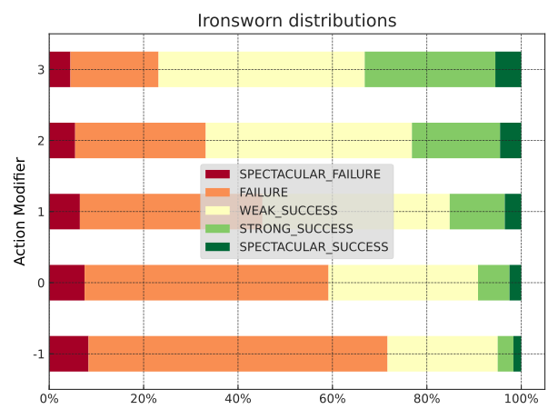
Now for a twist. A failure or success is particularly spectacular when the d10s come up doubles. The doubles rule uses both challenge-die outcomes. To model it, evaluate each combination of outcomes from the modified d6 and both d10s.

expand evaluates combinations from multiple source histograms or pools.

from enum import IntEnum

from dyce import H, HResult, PResult, expand
from dyce.d import d6, p2d10

class IronDramaticResult(IntEnum):
    SPECTACULAR_FAILURE = -1
    FAILURE = 0
    WEAK_SUCCESS = 1
    STRONG_SUCCESS = 2
    SPECTACULAR_SUCCESS = 3

    def __repr__(self) -> str:
        return self.name

def iron_dramatic_dependent_term(
    action: HResult[int],
    challenges: PResult[int],
    *,
    action_mod: int = 0,
) -> IronDramaticResult:
    modded_act = action.outcome + action_mod
    assert len(challenges.roll) == 2, "pool must have exactly 2 challenge dice"
    ch1_outcome, ch2_outcome = challenges.roll
    doubles = ch1_outcome == ch2_outcome
    modded_act_beats_ch1 = modded_act > ch1_outcome
    modded_act_beats_ch2 = modded_act > ch2_outcome
    if modded_act_beats_ch1 and modded_act_beats_ch2:
        return (
            IronDramaticResult.SPECTACULAR_SUCCESS
            if doubles
            else IronDramaticResult.STRONG_SUCCESS
        )
    elif modded_act_beats_ch1 or modded_act_beats_ch2:
        return IronDramaticResult.WEAK_SUCCESS
    else:
        return (
            IronDramaticResult.SPECTACULAR_FAILURE
            if doubles
            else IronDramaticResult.FAILURE
        )

action_mods = list(range(-1, 4))
results_by_action_mod = {
    action_mod: expand(
        iron_dramatic_dependent_term, d6, p2d10, action_mod=action_mod
    )
    for action_mod in action_mods
}

The callback accepts mod as a keyword-only parameter, which lets us pass values to it through expand for visualization.

Table:

import pandas as pd

data = [
    {
        outcome.name: float(prob)
        for outcome, prob in H.from_counts(
            result, dict.fromkeys(IronDramaticResult, 0), preserve_zero_counts=True
        ).probability_items()
    }
    for result in results_by_action_mod.values()
]

df = pd.DataFrame(data, index=action_mods)
df.index.name = "Action Modifier"

	SPECTACULAR_FAILURE	FAILURE	WEAK_SUCCESS	STRONG_SUCCESS	SPECTACULAR_SUCCESS
Action Modifier
-1	8.33%	63.33%	23.33%	3.33%	1.67%
0	7.50%	51.67%	31.67%	6.67%	2.50%
1	6.50%	38.67%	39.67%	11.67%	3.50%
2	5.50%	27.67%	43.67%	18.67%	4.50%
3	4.50%	18.67%	43.67%	27.67%	5.50%

Visualization:

import matplotlib.ticker as mticker

ax = df.plot(kind="barh", stacked=True, colormap="RdYlGn")
ax.xaxis.set_major_formatter(mticker.PercentFormatter(xmax=1))
ax.set_title("Ironsworn distributions")
ax.legend(loc="center")

Plot: Ironsworn distributions

Interactive version: